7 Changing Bases, Canonical Forms and Symmetries

7.1 Changing Bases in General

7.1.1 Definition and Proposition

Recall Matrices for Linear Maps in General given linear map $T : V \to W$ (real or complex vector spaces) and choice of bases \[\begin{align*} \{\underline{e}_i\} \hspace{0.5cm} i &= 1, \dots, n \text{ for } V \\ \{\underline{f}_a\} \hspace{0.5cm} a &= 1, \dots, m \text{ for } W \end{align*}\] the matrix $A$ ($m \times n$) w.r.t these bases is defined by \[\begin{align*} T(\underline{e}_i) &= \sum_a \underline{f}_a A_{ai}. \end{align*}\]

This definition is chosen to ensure \[\begin{align*} \underline{y} = T(\underline{x}) \iff y_a &= \sum_i A_{ai} x_i \\ &= A_{ai} x_i \ (\sum \text{ convention}) \\ \text{where } \underline{x} = \sum_i x_i \underline{e}_i,\ \underline{y} &= \sum_a y_a \underline{f}_a \\ \text{which holds since } T\left(\sum_i x_i \underline{e}_i \right) &= \sum_i x_i T(\underline{e}_i) \\ &= \sum_i x_i \left( \sum_a \underline{f}_a A_{ai} \right) \\ &= \sum_a \underbrace{\left( \sum_i A_{ai} x_i \right)}_{y_a} \underline{f}_a. \end{align*}\] The same linear map $T$ has matrix $A'$ w.r.t bases \[\begin{align*} \{\underline{e}'_i\} \hspace{0.5cm} i &= 1, \dots, n \text{ for } V \\ \{\underline{f}'_a\} \hspace{0.5cm} a &= 1, \dots, m \text{ for } W \end{align*}\] defined by \[\begin{align*} T(\underline{e}'_i) &= \sum_a \underline{f}'_a A'_{ai}. \end{align*}\] To relate $A$ and $A'$ we need to say how bases are related, and change of base matrices $P$ ($n \times n$) and $Q$ ($m \times m$) are defined by \[\begin{align*} \underline{e}'_i &= \sum_j \underline{e}_j P_{ji},\ \underline{f}'_a = \sum_b \underline{f}_b Q_{ba} \end{align*}\] Note: $P$ and $Q$ are invertible; in relation above we can exchange $\underline{e}_i$ and $\underline{e}'_i$ with $P \to P^{-1}$ and similarly for $Q$.

Proposition 7.1 With definitions as above \[\begin{align*} A' = Q^{-1} A P \end{align*}\] which is the change of basis formula for matrix of a linear map.¹⁴

Example 7.1 $n = 2,\ m = 3$ \[\begin{align*} T(\underline{e}_1) &= \underline{f_1} + 2 \underline{f}_2 - \underline{f}_3 = \sum_a \underline{f}_a A_{a 1} \\ T(\underline{e}_2) &= -\underline{f_1} + 2 \underline{f}_2 + \underline{f}_3 = \sum_a \underline{f}_a A_{a 2} \\ \implies A &= \begin{pmatrix}1 & -1 \\2 & 2 \\-1 & 1\end{pmatrix} \end{align*}\] New basis for $V$ \[\begin{align*} \underline{e}'_1 &= \underline{e}_1 - \underline{e}_2 = \sum_i \underline{e}_i P_{i 1} \\ \underline{e}'_2 &= \underline{e}_1 + \underline{e}_2 = \sum_i \underline{e}_i P_{i 2} \\ \implies P &= \begin{pmatrix}1 & 1 \\-1 & 1\end{pmatrix} \end{align*}\] New basis for $W$ \[\begin{align*} \underline{f}'_1 &= \underline{f}_1 - \underline{f}_3 = \sum_i \underline{e}_i P_{i 1} \\ \underline{f}'_2 &= \underline{f}_2 = \sum_i \underline{e}_i P_{i 2} \\ \underline{f}'_3 &= \underline{f}_1 + \underline{f}_3 = \sum_i \underline{e}_i P_{i 3} \\ \implies Q &= \begin{pmatrix} 1 & 0 & 1 \\ 0 & 1 & 0 \\ -1 & 0 & 1 \end{pmatrix} \end{align*}\] Change of basis formula: \[\begin{align*} A' &= Q^{-1} A P \\ &= \begin{pmatrix} \frac{1}{2} & 0 & -\frac{1}{2} \\ 0 & 1 & 0 \\ \frac{1}{2} & 0 & \frac{1}{2} \end{pmatrix} \begin{pmatrix}1 & -1 \\2 & 2 \\-1 & 1\end{pmatrix} \begin{pmatrix}1 & 1 \\-1 & 1\end{pmatrix} \\ &= \begin{pmatrix}2 & 0 \\4 & 0 \\0 & 0\end{pmatrix}. \end{align*}\] Direct check: \[\begin{align*} T(\underline{e}'_1) &= 2 \underline{f}'_1 \\ T(\underline{e}'_2) &= 4 \underline{f}'_2 \ \checkmark. \end{align*}\]

7.1.2 Proof of proposition

Proof. \[\begin{align*} T(\underline{e}'_i) &= T\left( \sum_j \underline{e}_j P_{ji} \right) \ \text{ definition of $P$} \\ &= \sum_j T(\underline{e}_j) P_{ji} \ \text{ linearity of $T$} \\ &= \sum_j \sum_a \underline{f}_a A_{aj} P_{ji} \ \text{ definition of $A$} \\ T(\underline{e}'_i) &= \sum_b \underline{f}'_b A'_{bi} \ \text{definition of $A'$} \\ &= \sum_b \sum_a \underline{f}_a Q_{ab} A'_{bi} \ \text{ definition of $Q$} \end{align*}\] Comparing coefficients of $\underline{f}_a$ as it is a basis \[\begin{align*} \sum_j A_{aj} P_{ji} = \sum_b Q_{ab} A'_{bi} \\ \text{or } AP = QA'. \end{align*}\]

7.1.3 Approach using vector components

Consider \[\begin{align*} \underline{x} &= \sum_j x_j \underline{e}_j \\ &= \sum_i x'_i \underline{e}'_i \\ &= \sum_j \left( \sum_i P_{ji} x'_i \right) \underline{e}_j \\ \implies x_j &= P_{ji} x'_i \\ \text{Write } X &= \begin{pmatrix}x_1 \\\vdots \\x_n\end{pmatrix},\ X' = \begin{pmatrix}x'_1 \\ \vdots \\ x'_n \end{pmatrix} \\ \text{then } X &= PX' \text{ or } X' = P^{-1} X \end{align*}\] Note: some care needed if $V = \mathbb{R}^n$, e.g. $n = 2$ with $\underline{e}_1 = \begin{pmatrix}1 \\1\end{pmatrix},\ \underline{e}_2 = \begin{pmatrix}1 \\-1\end{pmatrix}$ then $\underline{x} = \begin{pmatrix}5 \\1\end{pmatrix} \in \mathbb{R}^2$ has $\underline{x} = 3 \underline{e}_1 + 2 \underline{e}_2$ so $X = \begin{pmatrix}3 \\2\end{pmatrix}$.
Similarly \[\begin{align*} \underline{y} &= \sum_b y_j \underline{f}_b \\ &= \sum_a y'_a \underline{f}'_a \\ \implies y_b &= Q_{ba} y'_a \\ \text{Then } Y &= QY' \text{ or } Y' = Q^{-1} Y \\ \text{where } Y &= \begin{pmatrix}y_1 \\\vdots \\y_m \end{pmatrix},\ Y' = \begin{pmatrix}y'_1 \\ \vdots \\ y'_m \end{pmatrix} \end{align*}\] Now, matrices $A, A'$ are defined to ensure $Y = AX$ and $Y' = A' X'$.

\[\begin{align*} \text{But } Y' &= Q^{-1} Y = Q^{-1} A X \\ &= (Q^{-1} A P) X' \\ &= A' X' \end{align*}\] which is true $\forall \; \underline{x}$, so $A' = Q^{-1} A P$.

7.1.4 Comments

Definition of matrix $A$ for $T : V \to W$ w.r.t. bases $\{ \underline{e}_i \}$ and $\{ \underline{f}_a \}$ can be expressed: column $i$ of $A$ consists of components of $T(\underline{e}_i)$ w.r.t. basis $\{ \underline{f}_a \}$ [For $T : \mathbb{R}^n \to \mathbb{R}^m$ with standard bases, columns of $A$ are images of standard basis vectors].
Similarly, definitions of $P$ and $Q$ say: columns consist of components of new basis vectors w.r.t. old.
With $V = W$ and same bases and $\underline{e}_i = \underline{f}_i,\ \underline{e}'_i = \underline{f}'_i$ we have $P = Q$ and $A' = P^{-1} A P$. Matrices representing the same linear map w.r.t. different bases are similar; conversely if $A$ and $A'$ are similar then we can regard them as representing the same linear map with $P$ defining the change of basis.
In Diagonalisability and Similarity we observed \[\begin{align*} \operatorname{tr}(A') &= \operatorname{tr}(A) \\ \det(A') &= \det A \\ \chi_{A'}(t) &= \chi_A(t) \end{align*}\] so these are properties of the linear map.
$V = W = \mathbb{R}^n$ or $\mathbb{C}^n$, with $\underline{e}_i$ the standard basis - matrix $A$ is diagonalisable iff $\exists$ basis of eigenvectors $\underline{e}'_i = \underline{v}_i$ with $A \underline{v}_i = \lambda_i \underline{v}_i$ (not $\sum$) and then $A' = P^{-1} A P = D = \begin{pmatrix}\lambda_1 & & \\ & \ddots & \\ & & \lambda_n\end{pmatrix}$ and $\underline{v}_i = \sum_j \underline{e}_j P_{ji}$ so the eigenvectors are the columns of $P$.
Specialising further $A^\dagger = A \implies \exists$ basis of orthonormal eigenvectors $\underline{e}'_i = \underline{u}_i$ and $P^\dagger = P^{-1}$.

7.2 Jordan Canonical/ Normal Form

This results classifies $n \times n$ complex matrices up to similarity.

Proposition 7.2 Any $2 \times 2$ complex matrix $A$ is similar to one of the following:

$A' = \begin{pmatrix}\lambda_1 & 0 \\0 & \lambda_2\end{pmatrix}$ with $\lambda_1 \neq \lambda_2,\ \chi_A = (t - \lambda_1) (t - \lambda_2)$.
$A' = \begin{pmatrix}\lambda & 0 \\0 & \lambda\end{pmatrix}$ with $\chi_A = (t - \lambda)^2$.
$A' = \begin{pmatrix}\lambda & 1 \\0 & \lambda\end{pmatrix}$ with $\chi_A = (t - \lambda)^2$.

Proof. $\chi_A(t)$ has 2 roots over $\mathbb{C}$.

For distinct roots/ evals $\lambda_1, \lambda_2$ we have $M_1 = m_1 = M_2 = m_2 = 1$ and eigenvectors $\underline{v}_1, \underline{v}_2$ provide a basis. Hence $A' = P^{-1} A P$ where eigenvectors are columns of $P$.
For repeated root/ eval $\lambda$, if $M_\lambda = m_\lambda = 2$, then same argument applies.
For repeated root/ eval $\lambda$, with $M_\lambda = 2$ and $m_\lambda = 1$, let $\underline{v}$ be an eigenvector for $\lambda$ and $\underline{w}$ any linearly independent vector. Then \[\begin{align*} A \underline{v} &= \lambda \underline{v} \\ A \underline{w} &= \alpha \underline{v} + \beta \underline{w}. \end{align*}\] Matrix of map w.r.t basis $\{\underline{v}, \underline{w}\}$ is \[\begin{align*} \begin{pmatrix}\lambda & \alpha \\0 & \beta\end{pmatrix}. \end{align*}\] But $\beta = \lambda$ (otherwise we get case (i) with evals $\lambda, \beta$) and $\alpha \neq 0$ (otherwise case (ii)). Now set $\underline{u} = \alpha \underline{v}$ and note \[\begin{align*} A \underline{u} = \lambda \underline{u} \\ A \underline{w} = \underline{u} + \lambda \underline{w} \end{align*}\] so w.r.t. basis $\{ \underline{u}, \underline{w}\}$ matrix is \[\begin{align*} A' = \begin{pmatrix}\lambda & 1 \\0 & \lambda\end{pmatrix}. \end{align*}\]

Example 7.2 (using a slightly different approach) \[\begin{align*} A &= \begin{pmatrix}1 & 4 \\-1 & 5\end{pmatrix} \\ \implies \chi_A(t) &= (t - 3)^2 \\ A - 3 I &= \begin{pmatrix}-2 & 4 \\-1 & 2\end{pmatrix}. \end{align*}\] Choose $\underline{w} = \begin{pmatrix}1 \\0\end{pmatrix}$ which is not an eigenvector and then $\underline{u} = (A - 3I) \underline{w} = \begin{pmatrix}-2 \\-1\end{pmatrix}$. But $(A - 3I)^2 = 0$ by Cayley-Hamilton Theorem, 6.4, so $(A - 3I)^2 \underline{w} = (A - 3I) \underline{u} = 0$ so \[\begin{align*} A \underline{u} &= 3 \underline{u} \\ A \underline{w} &= \underline{u} + 3 \underline{w} \end{align*}\] so basis $\{ \underline{u}, \underline{w}\}$ gives Jordan Canonical Form. Check: $P = \begin{pmatrix}-2 & 1 \\-1 & 0\end{pmatrix} \implies P^{-1} = \begin{pmatrix}0 & -1 \\1 & -2\end{pmatrix}$ so $P^{-1} A P = \begin{pmatrix}3 & 1 \\0 & 3\end{pmatrix}$.

Generalisation to larger matrices can be considered, starting with $N = \begin{pmatrix}0 & 1 & & \\ & 0 & \ddots & \\ & & \ddots & 1 \\ & & & 0\end{pmatrix}$ ($n \times n$) when applied to standard basis vectors gives $\underline{e}_n \mapsto \underline{e}_{n-1} \mapsto \dots \mapsto \underline{e}_1 \mapsto \underline{0}$. Note $J = \lambda I + N$ then $\chi_J(t) = (\lambda - t)^n$ but $m_\lambda = 1$ ($M_\lambda = n$).

Theorem 7.1 Any $n \times n$ complex matrix $A$ is similar to a matrix $A'$ with block form \[\begin{align*} A' &= \begin{pmatrix} \boxed{J_{n_1}(\lambda_1)} & & & \\ & \boxed{J_{n_2}(\lambda_2)} & & \\ & & \ddots & \\ & & & \boxed{J_{n_r}(\lambda_r)} \end{pmatrix} \end{align*}\] where each diagonal block is a Jordan block with form \[\begin{align*} J_p(\lambda) &= \begin{pmatrix} \lambda & 1 & & & \\ & \lambda & 1 & & \\ & & \lambda & \ddots & \\ & & & \ddots & 1 \\ & & & & \lambda \end{pmatrix} \end{align*}\] ($p \times p$) with $n_1 + n_2 + \dots + n_r = n$, $\lambda_1, \lambda_2, \dots, \lambda_r$ are the eigenvalues of $A$ and $A'$ (same eigenvalue may appear in more than one block).

$A$ is diagonalisable iff $A'$ consists of $1 \times 1$ Jordan blocks only.

Proof. See Linear Algebra and GRM in Part IB.

7.3 Conics and Quadrics

7.3.1 Quadrics in General

Definition 7.1 (Quadric) A quadric in $\mathbb{R}^n$ is a hypersurface defined by \[\begin{align*} Q(\underline{x}) = \underline{x}^T A \underline{x} + \underline{b}^T \underline{x} + c = 0 \end{align*}\] for some $A$, $n \times n$ real symmetric, non-zero matrix, $\underline{b} \in \mathbb{R}^n$, $c \in \mathbb{R}$. So $Q(\underline{x}) = A_{ij} x_i x_j + b_i x_i + c = 0$.

Consider classifying solutions up to geometrical equivalence : no distinction between solutions related by isometries in $\mathbb{R}^n$, i.e. related by

translation - change in origin
orthogonal transformation about origin - change in the axes

If $A$ is invertible (no zero eigenvalues) then by setting $\underline{y} = \underline{x} + \frac{1}{2} A^{-1} \underline{b}$ we have \[\begin{align*} \underline{y}^T A \underline{y} &= (\underline{x} + \frac{1}{2}A^{-1} \underline{b})^T A (\underline{x} + \frac{1}{2}A^{-1} \underline{b}) \\ &= \underline{x}^T A \underline{x} + \underline{b}^T \underline{x} + \frac{1}{4} \underline{b}^T A^{-1} \underline{b} \end{align*}\] since $(A^{-1} \underline{b})^T = \underline{b}^T A^{-1}$ as $A$ is symmetric so $\frac{1}{2} (A^{-1} \underline{b})^T A \frac{1}{2} (A^{-1} \underline{b})$ is the last term.

Then $Q(\underline{x}) = 0 \iff \mathcal{F}(\underline{y}) = k$ with $\mathcal{F}(\underline{y}) = \underline{y}^T A \underline{y}$ (a quadratic form w.r.t. new origin $\underline{y} = 0$) and $k = \frac{1}{4} \underline{b}^T A^{-1} \underline{b} - c$. Diagonalise $\mathcal{F}$ as in Quadratic Forms: orthonormal eigenvectors give principal axes; eigenvalues of $A$ and value of $k$ determine nature of this quadric.

Examples in $\mathbb{R}^3$ given in In $\mathbb{R}^3$

eigenvalues $> 0$ and $k > 0$ give ellipsoid
eigenvalues have different signs and $k \neq 0$ gives a hyperboloid.

If $A$ has one or more zero eigenvalues then analysis changes and simplest standard form may have both linear and quadratic terms.

7.3.2 Conics

Quadrics in $\mathbb{R}^2$ are curves, conics.

If $\det A \neq 0$
By completing the square and diagonalising we get a standard form \[\begin{align*} \lambda_1 x_1'^2 + \lambda_2 x_2'^2 &= k \end{align*}\]
- $\lambda_1, \lambda_2 > 0 \implies$ ellipse for $k > 0$, point for $k = 0$ and no soln for $k < 0$.
- $\lambda_1 > 0, \lambda_2 < 0 \implies$ hyperbola for $k > 0$ or $k < 0$ and a pair of lines for $k = 0$.
  e.g. $x_1'^2 - x_2'^2 = (x_1 - x_2) (x_1 + x_2) = 0$.
If $\det A = 0$
Suppose $\lambda_1 > 0$ and $\lambda_2 = 0$; diagonalise $A$ in original formula to get \[\begin{align*} \lambda_1 x_1'^2 + b_1' x_1' + b_2' x_2' + c &= 0 \\ \iff \lambda_1 x_1''^2 + b_2' x_2' + c' &= 0 \end{align*}\] where $x_1'' = x_1' + \frac{1}{2 \lambda_1} b_1'$ and $c' = c - \frac{b_1'^2}{4 \lambda_1^2}$
- If $b_2' = 0$ we get a pair of lines for $c' < 0$, a single line for $c' = 0$ and no soln for $c' > 0$
- If $b_2' \neq 0$ equations becomes $\lambda_1 x_1''^2 + b_2 x_2'' = 0$, a parabola, where $x_2'' = x_2 + \frac{1}{b_2'}c'$.

7.4 Symmetries and Transformation Groups.

7.4.1 Orthogonal Transformations and Rotations in $\mathbb{R}^n$

\[\begin{align*} \underset{n \times n}{R} \text{ is orthogonal} &\iff R^T R = R R^T = I \\ &\iff (R \underline{x}) \cdot (R \underline{y}) = \underline{x} \cdot \underline{y} \ \forall \; \underline{x}, \underline{y} \\ &\iff \text{ cols or rows of $R$ are orthonormal vectors}. \end{align*}\] The set of such matrices forms the orthogonal group $O(n)$. \[\begin{align*} R \in O(n) \implies \det R = \pm 1. \end{align*}\] ($\det (R^T) \det R = (\det R)^2 = 1$).
$SO(n) = \{R \in O(n) : \det R = + 1\}$ is a subgroup, the special orthogonal group. $R \in O(n) \implies$ R preserves lengths and |n-dim volume|. $R \in SO(n) \implies$ R also preserves orientation. $SO(n)$ consists of all rotations in $\mathbb{R}^n$

Reflections belong to $O(n)$ but not $SO(n)$. For a specific $H \in O(n) \setminus SO(n)$, any element of $O(n)$ is of the form $R$ or $RH$ with $R \in SO(n)$, e.g. if $n$ is odd, we can choose $H = -I$.

7.4.1.1 Active and Passive points of View

For a rotation $R$ (matrix), the transformation \[\begin{align*} x_i' = R_{ij} x_j \end{align*}\] can be viewed in two ways.

Active view point: rotation transforms vectors, i.e. $x_i'$ are the components of the new vector so $\underline{x}' = R \underline{x}$ w.r.t. standard basis $\{ \underline{e}_i \}$.

Example 7.3 ($\mathbb{R}^2$)

$|\underline{x}'|^2 = |\underline{x}|^2$

Passive view point: rotation changes basis, i.e. $x_i'$ are the components of same vector $\underline{x}$ but w.r.t. new basis $\{\underline{u}_i\}$.

Example 7.4 ($\mathbb{R}^2$)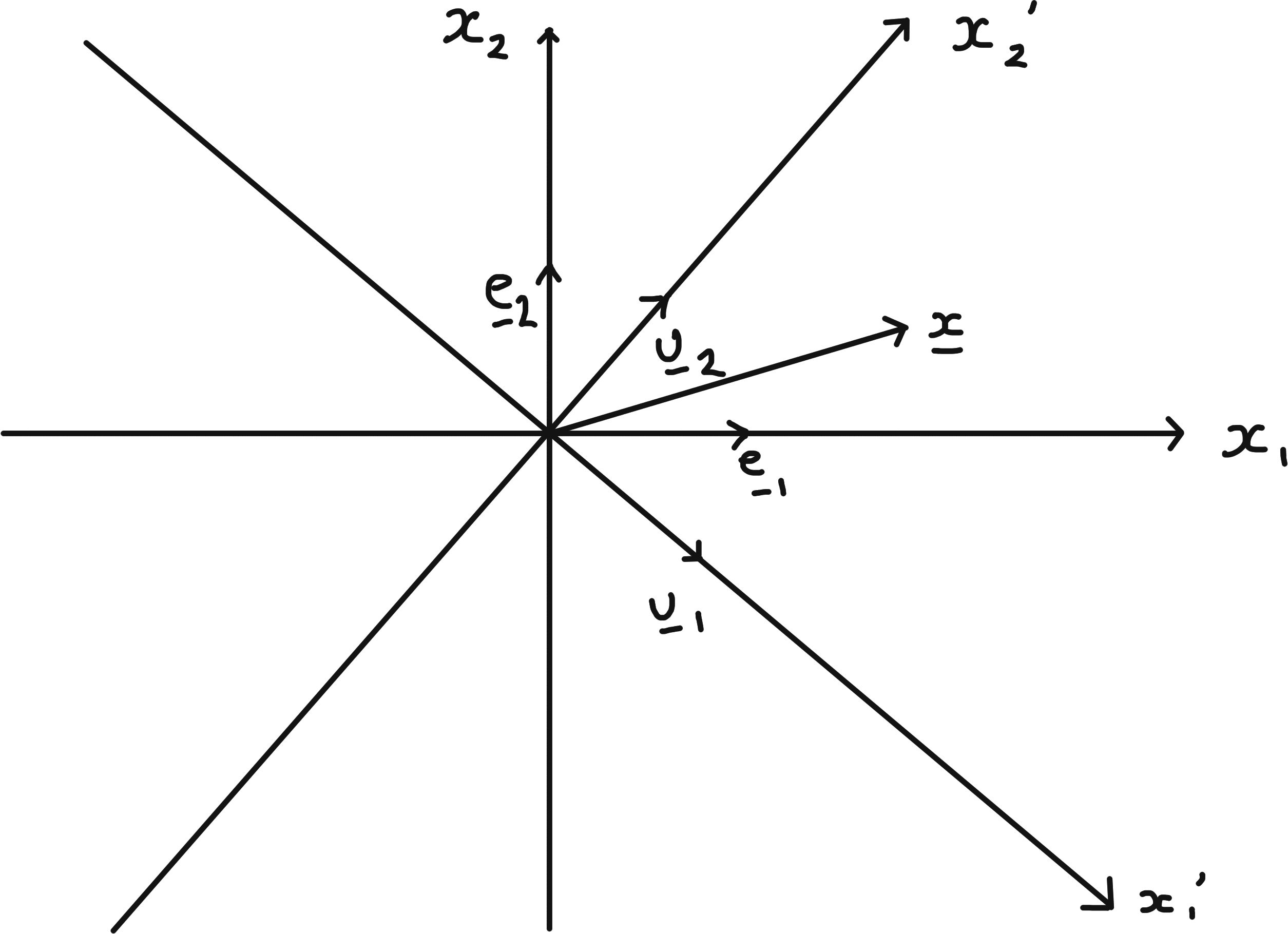

\[\begin{align*} \underline{u}_i &= \sum_j R_{ij} \underline{e}_j \\ &= \sum_J \underline{e}_j (R^T)_{ji} \\ &= \sum_J \underline{e}_j (R^{-1})_{ji} \end{align*}\] (compare to Quadratic Forms : $P = R^{-1}$).

7.4.2 2d Minkowski Space and Lorentz Transformations

Define a new “inner product” on $\mathbb{R}^2$ by \[\begin{align*} (\underline{x}, \underline{y}) = \underline{x}^T J \underline{y} \quad \text{where } J = \begin{pmatrix}1 & 0 \\0 & -1\end{pmatrix} \\ \therefore \left( \begin{pmatrix} x_0 \\ x_1 \end{pmatrix}, \begin{pmatrix} y_0 \\ y_1 \end{pmatrix} \right) = x_0 y_0 - x_1 y_1 \end{align*}\] This is not positive definite since $(\underline{x}, \underline{x}) = \underline{x}^T J \underline{x} = x_0^2 - x_1^2$ but still bilinear and symmetric. Standard basis vectors are “orthonormal” in generalised sense \[\begin{align*} \underline{e}_0 = \begin{pmatrix}1 \\0\end{pmatrix} &\text{ and } \underline{e}_1 = \begin{pmatrix}0 \\1\end{pmatrix} \\ \text{obey } (\underline{e}_0, \underline{e}_0) &= 1 \\ (\underline{e}_1, \underline{e}_1) &= -1 \\ (\underline{e}_0, \underline{e}_1) &= 0 \end{align*}\] This new inner product is called the Minkowski metric and $\mathbb{R}^2$ equipped with it is called Minkowski space.

Consider $M = \begin{pmatrix}M_{00} & M_{01} \\M_{10} & M_{11}\end{pmatrix}$ giving a linear map $\mathbb{R}^2 \to \mathbb{R}^2$. This preserves the Minkowski metric iff \[\begin{align*} (M \underline{x}, M \underline{y}) &= (\underline{x}, \underline{y}) \quad \forall \; x, y \in \mathbb{R}^2 \\ \iff (M \underline{x})^T J (M \underline{y}) &= \underline{x}^T (M^T J M) \underline{y} \\ &= \underline{x}^T J \underline{y} \quad \forall \; \underline{x}, \underline{y} \in \mathbb{R}^2 \\ \iff M^T J M &= J. \end{align*}\] The set of such matrices form a group. Now \[\begin{align*} \det (M^T J M) &= \det (M^T) \det J \det M \\ &= \det J \\ \implies (\det M)^2 &= 1 \implies \det M = \pm 1 \end{align*}\] Furthermore, $|M_{00}| \geq 1$, so $M_{00} \geq 1$ or $M_{00} \leq -1$. The subgroup with $\det M = + 1$ and $M_{00} \geq 1$ is the Lorentz group in 2d.

General form for $M$: require cols $M \underline{e}_0, M \underline{e}_1$ to be orthonormal w.r.t Minkowski metric, like $\underline{e}_0, \underline{e}_1$.

\[\begin{align*} (M \underline{e_0}, M \underline{e_0}) = M_{00}^2 - M_{10}^2 = (\underline{e_0}, \underline{e_0}) = 1 \quad (\text{hence } |M_{00}|^2 \geq 1) \end{align*}\]

Taking $M_{00} \geq 1$, we can write \[\begin{align*} M \underline{e_0} = \begin{pmatrix} \cosh \theta \\ \sinh \theta \end{pmatrix} \end{align*}\] for some real value $\theta$. For the other column, \[\begin{align*} (M \underline{e_0}, M \underline{e_1}) = 0;\; (M \underline{e_1}, M \underline{e_1}) = -1 \implies M \underline{e_1} = \pm \begin{pmatrix} \sinh \theta \\ \cosh \theta \end{pmatrix} \end{align*}\]¹⁵ The sign is fixed to be positive by the condition that $\det M = +1$. \[\begin{align*} M(\theta) = \begin{pmatrix} \cosh \theta & \sinh \theta \\ \sinh \theta & \cosh \theta \end{pmatrix} \end{align*}\] For such matrices \[\begin{align*} M(\theta_1) M(\theta_2) &= M(\theta_1 + M \theta_2). \end{align*}\] This confirms that they form a group.

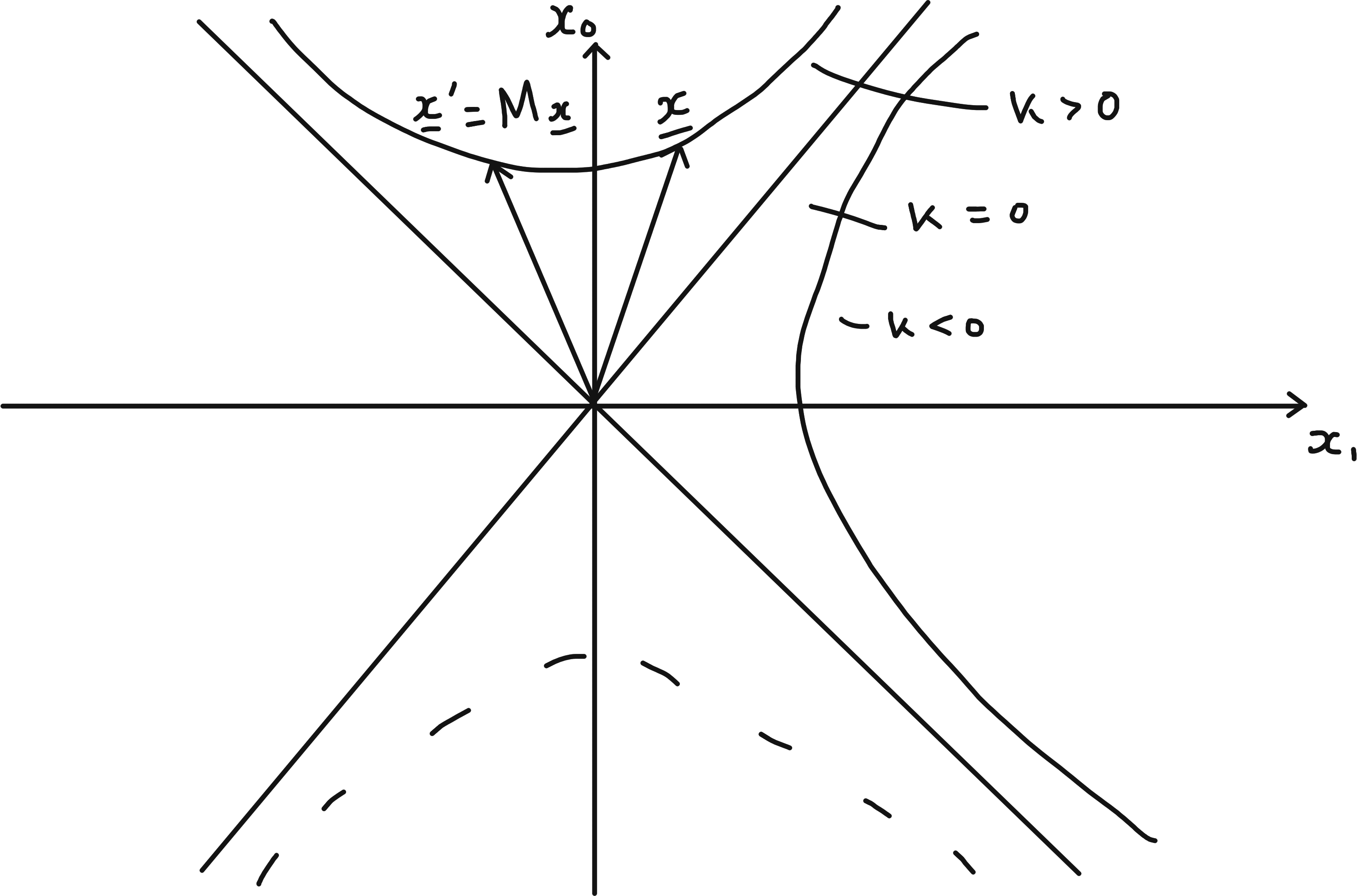
The curves defined by $(\underline{x}, \underline{x}) = k$ where $k$ is a constant are hyperbolas, as shown. This is analogous to how the curves defined by $\underline{x} \cdot \underline{x} = k$ are circles. So applying $M$ to any vector on a given branch of a hyperbola, the resultant vector remains on the hyperbola. Allowing $|M_{00}| < -1$ we would get transformations that could map $\underline{x}$ to the dotted branch below.

7.4.3 Application to special relativity

Set \[\begin{align*} M(\theta) &= \gamma(v) \begin{pmatrix} 1 & v \\ v & 1 \end{pmatrix} \\ v &= \tanh \theta,\quad |v| < 1 \\ \gamma(v) &= (1 - v^2)^{-\frac{1}{2}} \end{align*}\] We will rename $x_0 \to t$, which is now our time coordinate. $x_1 \to x$, our one-dimensional space coordinate. Then, \[ \underline{x}' = M \underline{x} \iff \begin{cases} t' & = \gamma(v) (t + vx) \\ x' & = \gamma(v) (x + vt) \end{cases} \] This is a Lorentz transformation or boost relating the time and space coordinates for observers moving with relative velocity $v$ in Special Relativity, in units where the speed of light $c$ is taken to be 1. The factor $\gamma$ gives rise to effects such as time dilation and length contraction.

The group property $M(\theta_3) = M(\theta_1)M(\theta_2)$ with $\theta_3 = \theta_1 + \theta_2$ corresponds to the velocities \[ v_i = \tanh \theta_i \implies v_3 = \frac{v_1 + v_2}{1 + v_1 v_2} \] This is consistent with the fact that all velocities are less than the speed of light, 1.

$P$ expresses our vector in $\underline{e}'_i$ the basis in terms of the $\underline{e}_i$ basis. E.g. $P * (1 \ 0 \dots \ 0)^T$ gives $P_{i 1} \underline{e}_i$ which is $\underline{e}'_1$ in terms of $\underline{e}_i$. Then we apply $A$ and get the components in terms of $\underline{f}_i$ so we use $Q^{-1}$ to convert to $\underline{f}'_i$.↩︎
for standard inner product to get normal vector swap $x$ and $y$ values and make one negative, here we don’t need to make one component negative.↩︎

Vectors and Matrices 2021 - 2022